Meta-analysis on Psilocybin for Depression
This document outlines the steps taken to perform a meta-analysis investigating the efficacy of psilocybin for treating depression, using data collated for the SYPRES project.
Load Packages
Next, we load the necessary R packages for data manipulation,
meta-analysis, and visualization. Key packages include: - readr and
tidyverse for data loading and manipulation. - meta and metafor
for conducting the meta-analysis calculations. - esc for effect size
calculation utilities. - metapsyTools for specialized functions
designed for psychiatric meta-analyses, particularly handling data
formats and running pre-defined analysis pipelines. - dmetar for
additional meta-analysis functions and tools.
library(readr)
library(tidyverse)
library(meta)
library(metafor)
library(esc)
library(metapsyTools)
library(dmetar)
Data Loading and Preparation
The raw data is loaded from a CSV file. This dataset contains information extracted from multiple studies.
Some studies report change scores from baseline rather than endpoint scores. To pool these studies with those reporting endpoint means and standard deviations (SDs), we need endpoint SDs for the change score studies. Where these are missing, we impute them.
Specifically, for the MADRS (Montgomery–Åsberg Depression Rating Scale)
outcome: 1. We identify studies reporting change scores
(outcome_type == "change"). 2. For Rosenblat et al. (2024) and Goodwin
et al. (2022), endpoint SDs are imputed using the average endpoint SD
from the Raison et al. (2023) study arms. We calculate the endpoint mean
by adding the mean change to the baseline mean. These rows are marked
with outcome_type = "imsd" (imputed mean/SD). 3. For Raison et
al. (2023) itself, we use the reported endpoint SDs directly and
calculate the endpoint means from the change scores and baseline means.
These rows retain outcome_type = "msd".
The original dataset is then combined with these new rows containing the calculated/imputed endpoint data.
Finally, we use functions from the metapsyTools package
(checkDataFormat and checkConflicts) to ensure the combined data
conforms to the expected structure and to identify potential
inconsistencies (e.g., differing control group data reported for the
same study).
# Load data
data <- read_csv("../data/data.csv")
## Rows: 291 Columns: 59
## ── Column specification ────────────────────────────────────────────────────────
## Delimiter: ","
## chr (28): study, condition_arm1, condition_arm2, multi_arm1, multi_arm2, out...
## dbl (30): primary_instrument, time_weeks, time_days, primary_timepoint, n_ar...
## lgl  (1): target_group
##
## ℹ Use `spec()` to retrieve the full column specification for this data.
## ℹ Specify the column types or set `show_col_types = FALSE` to quiet this message.
# Get baseline data for change studies' MADRS
change_data <- data %>%
  filterPoolingData(instrument == "madrs", outcome_type == "change")

# Use Raison endpoint SD for imputation
Raison_endpoint_sd_arm1 <- 13.04 # hard-coded for now
Raison_endpoint_sd_arm2 <- 12.51 # hard-coded for now
Raison_endpoint_sd_average <- (Raison_endpoint_sd_arm1 + Raison_endpoint_sd_arm2) / 2

# Create new rows based on change_data with outcome_type = "imsd" (imputed msd)
imsd_rows <- change_data %>%
  filterPoolingData(study %in% c("Rosenblat 2024", "Goodwin 2022")) %>%
  mutate(
    outcome_type = "imsd",
    sd_arm1 = Raison_endpoint_sd_average,
    sd_arm2 = Raison_endpoint_sd_average,
    mean_arm1 = mean_change_arm1 + baseline_m_arm1,
    mean_arm2 = mean_change_arm2 + baseline_m_arm2,
    n_arm1 = n_change_arm1,
    n_arm2 = n_change_arm2
  ) %>%
  mutate(
    sd_change_arm1 = NA,
    sd_change_arm2 = NA,
    mean_change_arm1 = NA,
    mean_change_arm2 = NA,
    n_change_arm1 = NA,
    n_change_arm2 = NA
  )
# Use individual SDs for Raison
Raison_rows <- change_data %>%
  filterPoolingData(study == "Raison 2023") %>%
  mutate(
    outcome_type = "msd",
    sd_arm1 = Raison_endpoint_sd_arm1,
    sd_arm2 = Raison_endpoint_sd_arm2,
    mean_arm1 = mean_change_arm1 + baseline_m_arm1,
    mean_arm2 = mean_change_arm2 + baseline_m_arm2,
    n_arm1 = n_change_arm1,
    n_arm2 = n_change_arm2
  ) %>%
  mutate(
    sd_change_arm1 = NA,
    sd_change_arm2 = NA,
    mean_change_arm1 = NA,
    mean_change_arm2 = NA,
    n_change_arm1 = NA,
    n_change_arm2 = NA
  )

# Append the new rows to the data dataframe
data <- bind_rows(data, imsd_rows, Raison_rows)

# Check data format with checkDataFormat
checkDataFormat(data)
## - [OK] Data set contains all variables in 'must.contain'.
## - [OK] 'study' has desired class character.
## - [OK] 'condition_arm1' has desired class character.
## - [OK] 'condition_arm2' has desired class character.
## - [OK] 'multi_arm1' has desired class character.
## - [OK] 'multi_arm2' has desired class character.
## - [OK] 'outcome_type' has desired class character.
## - [OK] 'instrument' has desired class character.
## - [OK] 'time' has desired class character.
## - [OK] 'time_weeks' has desired class numeric.
## - [OK] 'rating' has desired class character.
## - [OK] 'mean_arm1' has desired class numeric.
## - [OK] 'mean_arm2' has desired class numeric.
## - [OK] 'sd_arm1' has desired class numeric.
## - [OK] 'sd_arm2' has desired class numeric.
## - [OK] 'n_arm1' has desired class numeric.
## - [OK] 'n_arm2' has desired class numeric.
## - [OK] 'event_arm1' has desired class numeric.
## - [OK] 'event_arm2' has desired class numeric.
## - [OK] 'totaln_arm1' has desired class numeric.
## - [OK] 'totaln_arm2' has desired class numeric.

## # A tibble: 317 × 59
##    study        condition_arm1 condition_arm2 multi_arm1 multi_arm2 outcome_type
##    <chr>        <chr>          <chr>          <chr>      <chr>      <chr>
##  1 Rosenblat 2… psil           wl             <NA>       <NA>       change
##  2 Rosenblat 2… psil           wl             <NA>       <NA>       change
##  3 Rosenblat 2… psil           wl             <NA>       <NA>       change
##  4 Raison 2023  psil           ncn            <NA>       <NA>       change
##  5 Raison 2023  psil           ncn            <NA>       <NA>       change
##  6 Raison 2023  psil           ncn            <NA>       <NA>       change
##  7 Raison 2023  psil           ncn            <NA>       <NA>       change
##  8 Raison 2023  psil           ncn            <NA>       <NA>       change
##  9 Raison 2023  psil           ncn            <NA>       <NA>       change
## 10 Raison 2023  psil           ncn            <NA>       <NA>       change
## # ℹ 307 more rows
## # ℹ 53 more variables: instrument <chr>, rating <chr>,
## #   instrument_symptom <chr>, primary_instrument <dbl>, cov_time_point <chr>,
## #   time <chr>, time_weeks <dbl>, time_days <dbl>, primary_timepoint <dbl>,
## #   n_arm1 <dbl>, mean_arm1 <dbl>, sd_arm1 <dbl>, n_arm2 <dbl>,
## #   mean_arm2 <dbl>, sd_arm2 <dbl>, n_change_arm1 <dbl>,
## #   mean_change_arm1 <dbl>, sd_change_arm1 <dbl>, n_change_arm2 <dbl>, …
# Check conflicts with checkConflicts
checkConflicts(data)
## - [!] Data format conflicts detected!
## ID conflicts
## - check if variable(s) study, outcome_type, instrument, time, time_weeks, rating create(s) unique assessment point IDs
## - check if multi uniquely identifies all trial arms in multiarm trials
## --------------------

## Krempien 2023
Filter Data and Calculate Effect Sizes
Before running the main analysis, we prepare the data further:
- Calculate Effect Sizes: We use
calculateEffectSizes()(frommetapsyTools) to compute Hedges’ g (a standardized mean difference, SMD) and its standard error for each study comparison based on the endpoint means, SDs, and sample sizes. - Filter Data: We select the specific data points to be included
in the primary meta-analysis:
- Exclude specific low-dose arms (10 mg psilocybin) if present in multi-arm studies.
- Exclude the Krempien (2023) study.
- Use
filterPoolingData()(frommetapsyTools) to select only rows marked as the primary instrument (primary_instrument == "1") and primary timepoint (primary_timepoint == "1") for each study. - Include only the endpoint data (
outcome_type == "msd"or"imsd"), excluding the original change score data.
The resulting data_main dataframe contains the filtered data ready for
meta-analysis.
# Filter data to only include primary outcomes and timepoints
# Use filterPoolingData

data_main <- data %>%
  calculateEffectSizes() %>%
  filter(
    is.na(multi_arm1) | !str_detect(multi_arm1, "10 mg"),
    is.na(multi_arm2) | !str_detect(multi_arm2, "10 mg"),
    !str_detect(study, "Krempien 2023")
  ) %>%
  filterPoolingData(
    primary_instrument == "1",
    primary_timepoint == "1",
    outcome_type == "msd" | outcome_type == "imsd"
  )
## - [OK] Hedges' g calculated successfully.

## - [OK] Log-risk ratios calculated successfully.
Run Primary Meta-Analysis
We now perform the main meta-analysis using the runMetaAnalysis
function from metapsyTools. This function simplifies running standard
meta-analytic models.
We specify: - which.run = "overall": Conducts a random-effects
meta-analysis pooling all studies in data_main. - es.measure = "g":
Uses the pre-calculated Hedges’ g effect sizes. - method.tau = "REML":
Employs the Restricted Maximum Likelihood estimator for the
between-study variance (τ²). - hakn = TRUE: Applies the Knapp-Hartung
adjustment for significance tests, which is recommended for
meta-analyses with a small number of studies. - Various *.var
arguments map the columns in data_main to the required inputs for the
analysis (study labels, arm conditions, sample sizes, etc.).
The results, including the pooled effect size, confidence intervals,
heterogeneity statistics, and the meta-analysis model object, are stored
in main_results.
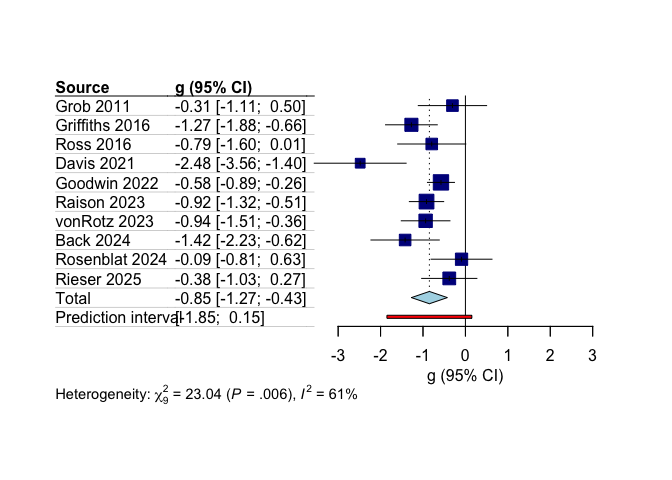
Finally, a basic forest plot is generated using meta::forest to
visualize the individual study effect sizes and the overall pooled
result. The studies are sorted by year.
main_results <- runMetaAnalysis(data_main, # using pre-filtered data for now

  # specify statistical parameters
  which.run = "overall", # inverse variance random effects
  es.measure = "g", # uses .g column in data_es and .g_se (Hedges' g/bias-corrected SMD)
  method.tau = "REML", # default, but still including for clarity
  method.tau.ci = "Q-Profile", # not sure if this will work!
  hakn = TRUE, # Knapp-Hartung effect size significance tests be used

  # specify variables in data_es
  study.var = "study",
  arm.var.1 = "condition_arm1",
  arm.var.2 = "condition_arm2",
  measure.var = "instrument",
  w1.var = "n_arm1",
  w2.var = "n_arm2",
  time.var = "time_weeks",
  round.digits = 2 # can change to change number of digits to round the presented results to
)
## - Running meta-analyses...

## - [OK] Using Hedges' g as effect size metric...

## - [OK] Calculating overall effect size... DONE
meta::forest(
  main_results$model.overall,
  sortvar = main_results$model.overall$data$year,
  layout = "JAMA"
)