Reproducibility Guide: Meta-analysis on MDMA for PTSD
This document provides a comprehensive walk-through of the meta-analysis investigating the efficacy of MDMA for treating PTSD symptoms, using data extracted for the SYPRES project. The analysis includes both continuous (PTSD symptom severity scores) and dichotomous (response/remission rates) outcomes, along with extensive subgroup and sensitivity analyses.
Our database for this analysis can be accessed through the R package
metapsyData. It can also be downloaded directly as a CSV file
here.
Documentation on metapsyData is available
here.
The meta-analytic portion of this script primarily uses the R package
metapsyTools. Documentation on metapsyTools is available
here.
This walk-through has some code chunks hidden for clarity. Full source code for this analysis is available here.
Overview
This meta-analysis synthesizes evidence from randomized controlled trials examining the efficacy of MDMA for treating PTSD. The analysis employs meta-analytic methods to provide robust estimates of treatment effects while accounting for study heterogeneity and potential biases.
Key Features of This Analysis
- Comprehensive outcome assessment: Both continuous (PTSD symptom severity) and dichotomous (response/remission) outcomes
- Dose-response analysis: Three-level hierarchical models to examine treatment effects with respect to dosing
- Co-morbid depression: Analysis of self-reported depression symptoms in PTSD
- Robustness testing: Extensive sensitivity analyses
- Publication bias assessment: Multiple methods to evaluate potential bias
- Transparent reporting: Complete code and methodology documentation
Methods
Key statistical specifications:
- Effect size: Hedges’ g for continuous outcomes, log RR for dichotomous outcomes
- Heterogeneity estimator: REML for random-effects models
- Confidence intervals: Q-Profile method for heterogeneity, Knapp-Hartung adjustment for effect sizes
- Significance testing: Knapp-Hartung adjustment for small sample sizes
Quality Assessment
Risk of bias was evaluated using the Cochrane Risk of Bias 2.0 tool. Publication bias is evaluated using a funnel plot and Egger’s test.
Load Required Packages
We begin by loading the necessary R packages for data manipulation, meta-analysis, and visualization:
- Data manipulation:
readrandtidyversefor data loading and manipulation - Meta-analysis:
metaandmetaforfor conducting meta-analytic calculations - Effect sizes:
escfor effect size calculation utilities - Specialized tools:
metapsyToolsfor specific meta-analysis functions anddmetarfor additional meta-analysis tools
library(readr)
library(tidyverse)
library(meta)
library(metafor)
library(metapsyTools)
library(metapsyData)
library(gt)
library(dmetar)
library(bayesmeta)
Data Loading and Quality Checks
The sypres database ptsd-mdmactr is downloaded using the metapsyData
package. Before proceeding with the analysis, we perform quality checks
to ensure data integrity and identify potential issues.
# Load data using metapsyData
d <- getData("ptsd-mdmactr")
data <- d$data


# Check data format with checkDataFormat
checkDataFormat(data)

# Check conflicts with checkConflicts
checkConflicts(data,
  vars.for.id = c(
    "study", "outcome_type",
    "instrument", "study_time_point",
    "time_weeks",
    "rating"
  )
)
# data <- read_csv2("~/Documents/GIT/data-ptsd-mdmactr/data.csv") # for parker
# data <- read_csv2("/Users/bsevchik/Documents/GitHub/data-ptsd-mdmactr/data.csv") # for brooke
data <- data %>%
  calculateEffectSizes(
    vars.for.id = c(
      "study", "outcome_type",
      "instrument", "study_time_point",
      "time_weeks",
      "rating"
    ),
  )
Data Preparation and Filtering
We prepare the data for analysis by applying several filters to create our primary analysis dataset:
- Primary outcomes: Select only the primary instrument and timepoint for each study
- Study design: Exclude post-crossover data
- Outcome type: Include only endpoint data (mean/SD/N)
- Dosing: Exclude medium-dose arms from multi-arm studies (Mithoefer 2018, Ot’alora 2018)
The resulting data_main dataframe contains the filtered data ready for
our primary meta-analysis.
data_main <- data %>%
  filterPoolingData(
    primary_instrument == "1",
    primary_timepoint == "1",
    is.na(post_crossover) | !Detect(post_crossover, "1"),
    outcome_type == "msd",
    !(Detect(study, "Mithoefer 2018") & (!is.na(multi_arm1)) & Detect(multi_arm2, "75 mg")),
    !(Detect(study, "Mithoefer 2018") & (Detect(multi_arm1, "75 mg") & !is.na(multi_arm2))),
    !(Detect(study, "Ot'alora 2018") & (!is.na(multi_arm1)) & Detect(multi_arm2, "100 mg")),
    !(Detect(study, "Ot'alora 2018") & (Detect(multi_arm1, "100 mg") & !is.na(multi_arm2)))
  )
Results
Primary Meta-Analysis
We conduct the main meta-analysis using the runMetaAnalysis function
from metapsyTools. This analysis pools all studies in our filtered
dataset to estimate the overall effect of MDMA on PTSD severity.
Key specifications:
-
Effect size: Hedges’ g (standardized mean difference)
-
Model: Random-effects meta-analysis using REML estimator
-
Adjustments: Knapp-Hartung adjustment for significance tests
The results include the pooled effect size, confidence intervals, heterogeneity statistics, and the meta-analysis model object.
# Run meta-analysis

main_results <- runMetaAnalysis(data_main,
  which.run = c("overall"),

  # Specify statistical parameters
  es.measure = "g", # Hedges' g
  method.tau = "REML",
  method.tau.ci = "Q-Profile",
  hakn = TRUE, # Knapp-Hartung adjustment

  # Specify variables
  study.var = "study",
  arm.var.1 = "condition_arm1",
  arm.var.2 = "condition_arm2",
  measure.var = "instrument",
  w1.var = "n_arm1",
  w2.var = "n_arm2",
  time.var = "time_days",
  round.digits = 2
)

summary(main_results$model.overall)
##                      g             95%-CI %W(random)
## Mitchell 2021  -0.7712 [-1.2295; -0.3129]       33.3
## Mitchell 2023  -0.5915 [-1.0069; -0.1760]       40.5
## Mithoefer 2011 -1.2080 [-2.1842; -0.2317]        7.3
## Mithoefer 2018 -0.9603 [-1.9458;  0.0251]        7.2
## Oehen 2013     -0.8525 [-2.1083;  0.4033]        4.4
## Ot'alora 2018  -0.2761 [-1.2607;  0.7084]        7.2
##
## Number of studies: k = 6
##
##                                 g             95%-CI     t p-value
## Random effects model (HK) -0.7119 [-0.9534; -0.4704] -7.58  0.0006
## Prediction interval               [-1.0588; -0.3651]
##
## Quantifying heterogeneity (with 95%-CIs):
##  tau^2 = 0 [0.0000; 0.3800]; tau = 0 [0.0000; 0.6164]
##  I^2 = 0.0% [0.0%; 74.6%]; H = 1.00 [1.00; 1.99]
##
## Test of heterogeneity:
##     Q d.f. p-value
##  2.42    5  0.7879
##
## Details of meta-analysis methods:
## - Inverse variance method
## - Restricted maximum-likelihood estimator for tau^2
## - Q-Profile method for confidence interval of tau^2 and tau
## - Calculation of I^2 based on Q
## - Hartung-Knapp adjustment for random effects model (df = 5)
## - Prediction interval based on t-distribution (df = 5)
# Create simple forest plot of results

plot(
  main_results,
  which = "overall"
)
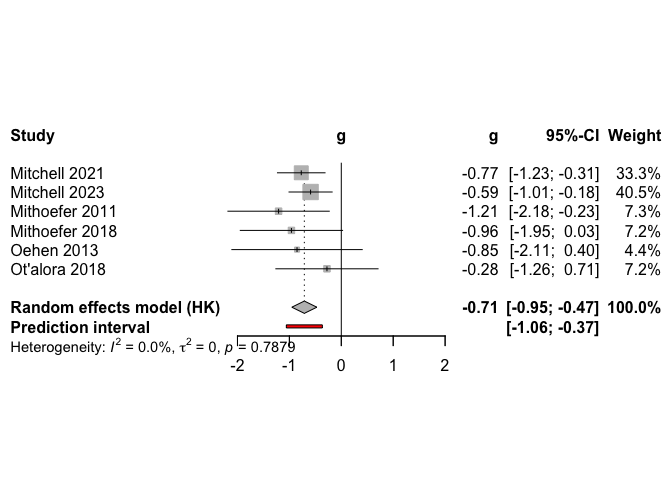
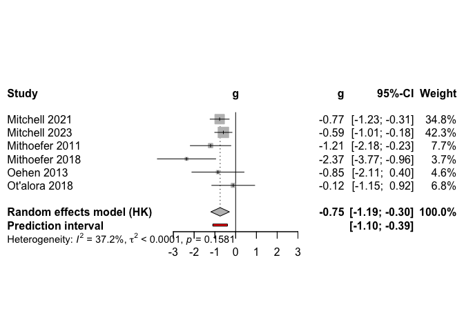
The primary meta-analysis on continuous outcomes in the 6 studies included in the main model showed a statistically significant reduction in PTSD scores with MDMA treatment as compared to control conditions, with small between-study heterogeneity.
Publication Bias Assessment
We assess potential publication bias using both visual (funnel plot) and statistical (Egger’s test) methods.
# Run Egger's test
eggers.test(main_results$model.overall)
## Warning in eggers.test(main_results$model.overall): Your meta-analysis contains k = 6 studies. Egger's test
## may lack the statistical power to detect bias when the number of studies is small (i.e., k<10).

## Eggers' test of the intercept
## =============================
##
##  intercept       95% CI      t         p
##     -0.517 -1.94 - 0.91 -0.712 0.5158656
##
## Eggers' test does not indicate the presence of funnel plot asymmetry.
Egger’s test did not indicate small-study effects/publication bias.
png(filename = file.path(basedir, "analysis/mdmaptsd/paperfigs/final/SI_Fig_01.png"), res = 315, width = 2500, height = 1500)
funnel(main_results$model.overall,
  studlab = TRUE, # can also use vector with study labels
  cex.studlab = 0.7, # adjust size of study labels
  cex = 0.7, # axis tick labels and point size
  cex.axis = 0.7, # axis number label size
  cex.lab = 0.7, # axis title (xlab, ylab) size
  cex.main = 0.95, # main title size
  xlim = c(-3, 0.2),
  col = "steelblue",
  pch = 19, # bold solid circle
  bg = "white",
  xlab = "Standardized Mean Difference (SMD)",
  ylab = "Standard Error (SE)",
  main = "Funnel Plot of Main Model Continuous Outcomes",
  las = 1
)
dev.off()
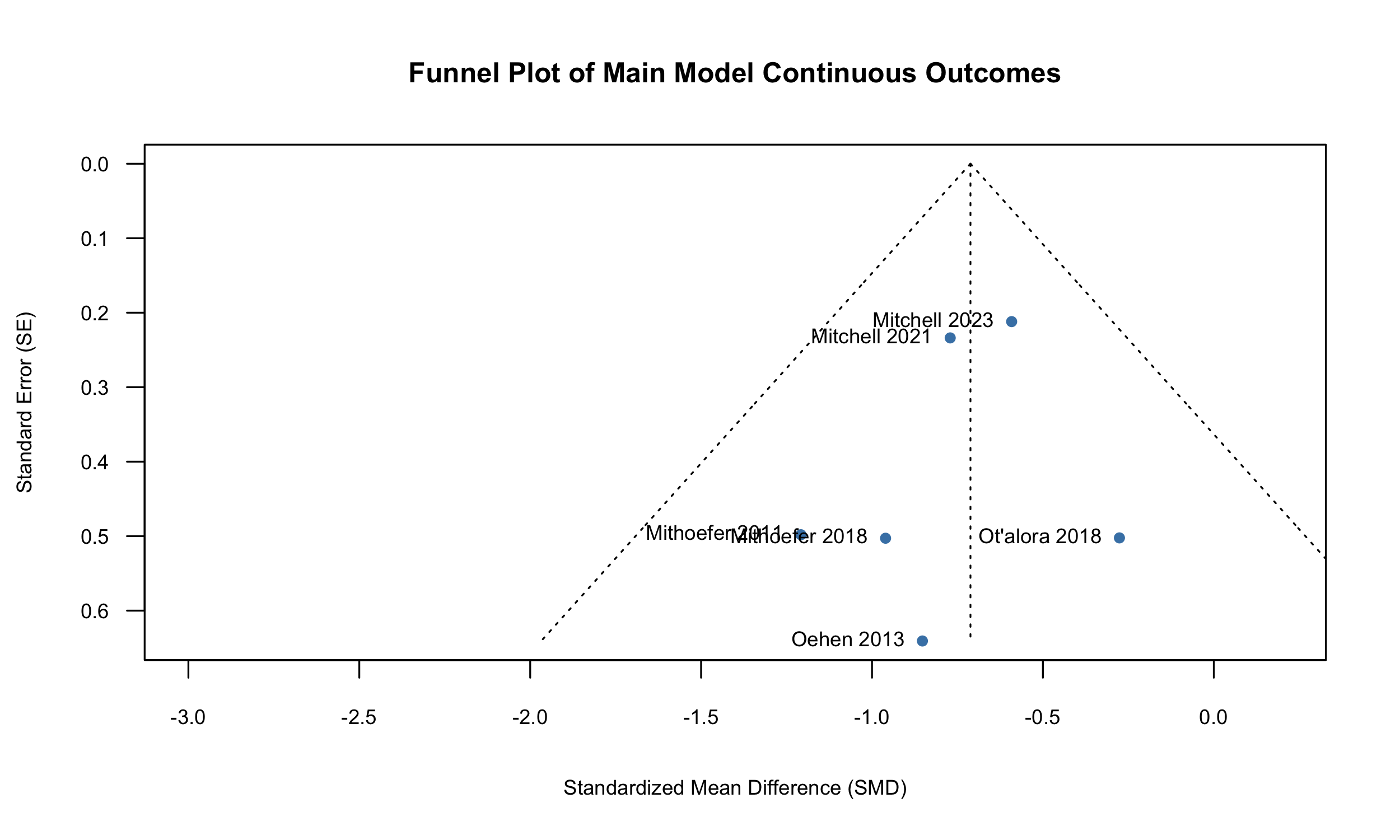 Visual inspection
of the funnel plot reveals limited asymmetry, and the Egger’s test did
not find small study effects, implying minimal evidence of publication
bias.
Visual inspection
of the funnel plot reveals limited asymmetry, and the Egger’s test did
not find small study effects, implying minimal evidence of publication
bias.
Three-level correlated and hierarchical effects (CHE) meta-analysis
We conduct a three-level correlated and hierarchical effects (CHE) meta-analysis to examine how the effect of MDMA changes over time. This approach accounts for the hierarchical structure of the data (multiple timepoints within studies) and potential correlations between timepoints.
# Select data for the CHE meta-analysis
data_time <- data %>%
  filterPoolingData(
    primary_instrument == "1",
    post_crossover == 0 | is.na(post_crossover),
    is.na(post_crossover) | !Detect(post_crossover, "1"),
    outcome_type == "msd",
    !(Detect(study, "Mithoefer 2018") & (!is.na(multi_arm1)) & Detect(multi_arm2, "75 mg")),
    !(Detect(study, "Ot'alora 2018") & (!is.na(multi_arm1)) & Detect(multi_arm2, "100 mg"))
  )

# Re-write some data for plotting
data_time$dose_arm1 <- as.numeric(gsub("mg", "", data_time$dose_arm1))
data_time$study[data_time$study == "Mithoefer 2018" & data_time$multi_arm1 == "75 mg"] <- "Mithoefer 2018 1"
data_time$study[data_time$study == "Mithoefer 2018" & data_time$multi_arm1 == "125 mg"] <- "Mithoefer 2018 2"
data_time$study[data_time$study == "Ot'alora 2018" & data_time$multi_arm1 == "100 mg"] <- "Ot'alora 2018 1"
data_time$study[data_time$study == "Ot'alora 2018" & data_time$multi_arm1 == "125 mg"] <- "Ot'alora 2018 2"

time_results <- runMetaAnalysis(data_time,
  which.run = "threelevel.che",
  # Specify statistical parameters
  es.measure = "g", # Hedges' g
  method.tau = "REML",
  method.tau.ci = "Q-Profile", # N/A for three-level models
  # i2.ci.boot = TRUE, # Need to use bootstrapping to get het. CI on three-level
  hakn = TRUE, # Knapp-Hartung adjustment

  # Specify variables
  study.var = "study",
  arm.var.1 = "condition_arm1",
  arm.var.2 = "condition_arm2",
  measure.var = "instrument",
  w1.var = "n_arm1",
  w2.var = "n_arm2",
  time.var = "dose_days",
  round.digits = 2
)

summary(time_results$model.threelevel.che)
##
## Multivariate Meta-Analysis Model (k = 15; method: REML)
##
##   logLik  Deviance       AIC       BIC      AICc
##  -8.9957   17.9914   23.9914   25.9086   26.3914
##
## Variance Components:
##
##             estim    sqrt  nlvls  fixed       factor
## sigma^2.1  0.0000  0.0000      8     no        study
## sigma^2.2  0.0253  0.1591     15     no  study/es.id
##
## Test for Heterogeneity:
## Q(df = 14) = 25.1579, p-val = 0.0330
##
## Model Results:
##
## estimate      se     tval  df    pval    ci.lb    ci.ub
##  -0.6034  0.1215  -4.9653  14  0.0002  -0.8640  -0.3428  ***
##
## ---
## Signif. codes:  0 '***' 0.001 '**' 0.01 '*' 0.05 '.' 0.1 ' ' 1
plot(
  time_results,
  which = "threelevel.che"
)
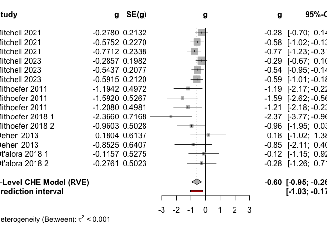
The three-level CHE model reveals an overall significant decrease in PTSD scores under MDMA compared to control conditions.
Meta-Regression
We perform two separate meta-regressions to examine the relationship between dose and treatment effect:
1. Number of dosing sessions
First, we examine the relationship between the number of dosing sessions and treatment effect.
reg <- metaRegression(time_results$model.threelevel.che, ~n_dosing_sessions)
reg
##
## Multivariate Meta-Analysis Model (k = 15; method: REML)
##
## Variance Components:
##
##             estim    sqrt  nlvls  fixed       factor
## sigma^2.1  0.0000  0.0000      8     no        study
## sigma^2.2  0.0000  0.0000     15     no  study/es.id
##
## Test for Residual Heterogeneity:
## QE(df = 13) = 16.1470, p-val = 0.2413
##
## Test of Moderators (coefficient 2):
## F(df1 = 1, df2 = 13) = 9.0109, p-val = 0.0102
##
## Model Results:
##
##                    estimate      se     tval  df    pval    ci.lb    ci.ub
## intrcpt             -0.1931  0.1728  -1.1176  13  0.2840  -0.5665   0.1802
## n_dosing_sessions   -0.1989  0.0663  -3.0018  13  0.0102  -0.3421  -0.0558  *
##
## ---
## Signif. codes:  0 '***' 0.001 '**' 0.01 '*' 0.05 '.' 0.1 ' ' 1
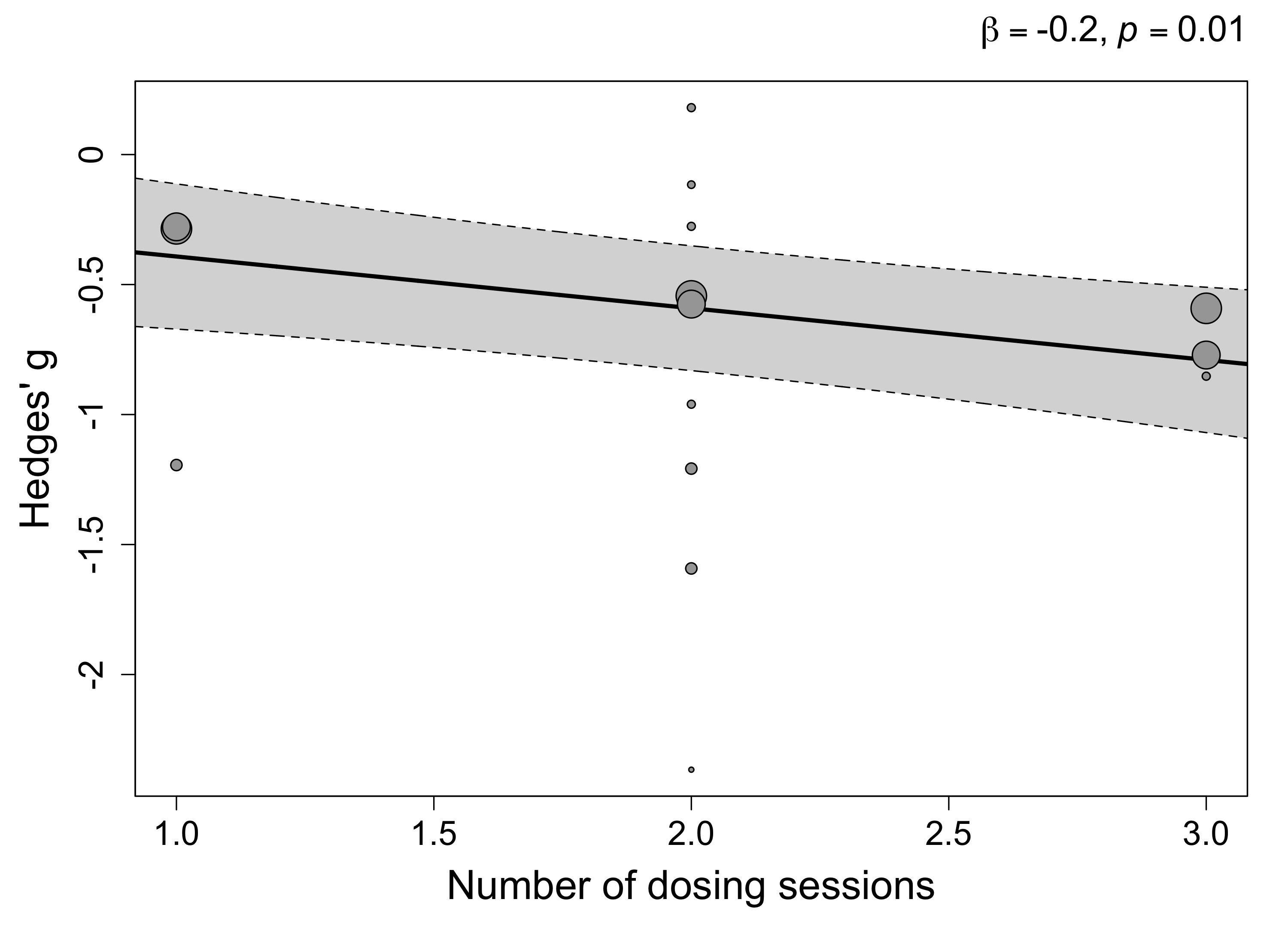
The largest between-group difference in PTSD scores occurs after the first dosing session (Hedges’ g = -0.39), while additional sessions increase this difference by -0.20 SMD.
2. Cumulative dose
We also examine the relationship between the cumulative dose and treatment effect. Cumulative dose is the total amount of MDMA taken by the participant (excluding booster doses for simplicity - all studies offered booster doses partway through the dosing sessions).
reg <- metaRegression(time_results$model.threelevel.che, ~cumulative_dose_arm1)
reg
##
## Multivariate Meta-Analysis Model (k = 15; method: REML)
##
## Variance Components:
##
##             estim    sqrt  nlvls  fixed       factor
## sigma^2.1  0.0000  0.0000      8     no        study
## sigma^2.2  0.0000  0.0000     15     no  study/es.id
##
## Test for Residual Heterogeneity:
## QE(df = 13) = 16.2583, p-val = 0.2355
##
## Test of Moderators (coefficient 2):
## F(df1 = 1, df2 = 13) = 8.8996, p-val = 0.0106
##
## Model Results:
##
##                       estimate      se     tval  df    pval    ci.lb    ci.ub
## intrcpt                -0.2495  0.1594  -1.5650  13  0.1416  -0.5939   0.0949
## cumulative_dose_arm1   -0.0016  0.0005  -2.9832  13  0.0106  -0.0028  -0.0005  *
##
## ---
## Signif. codes:  0 '***' 0.001 '**' 0.01 '*' 0.05 '.' 0.1 ' ' 1
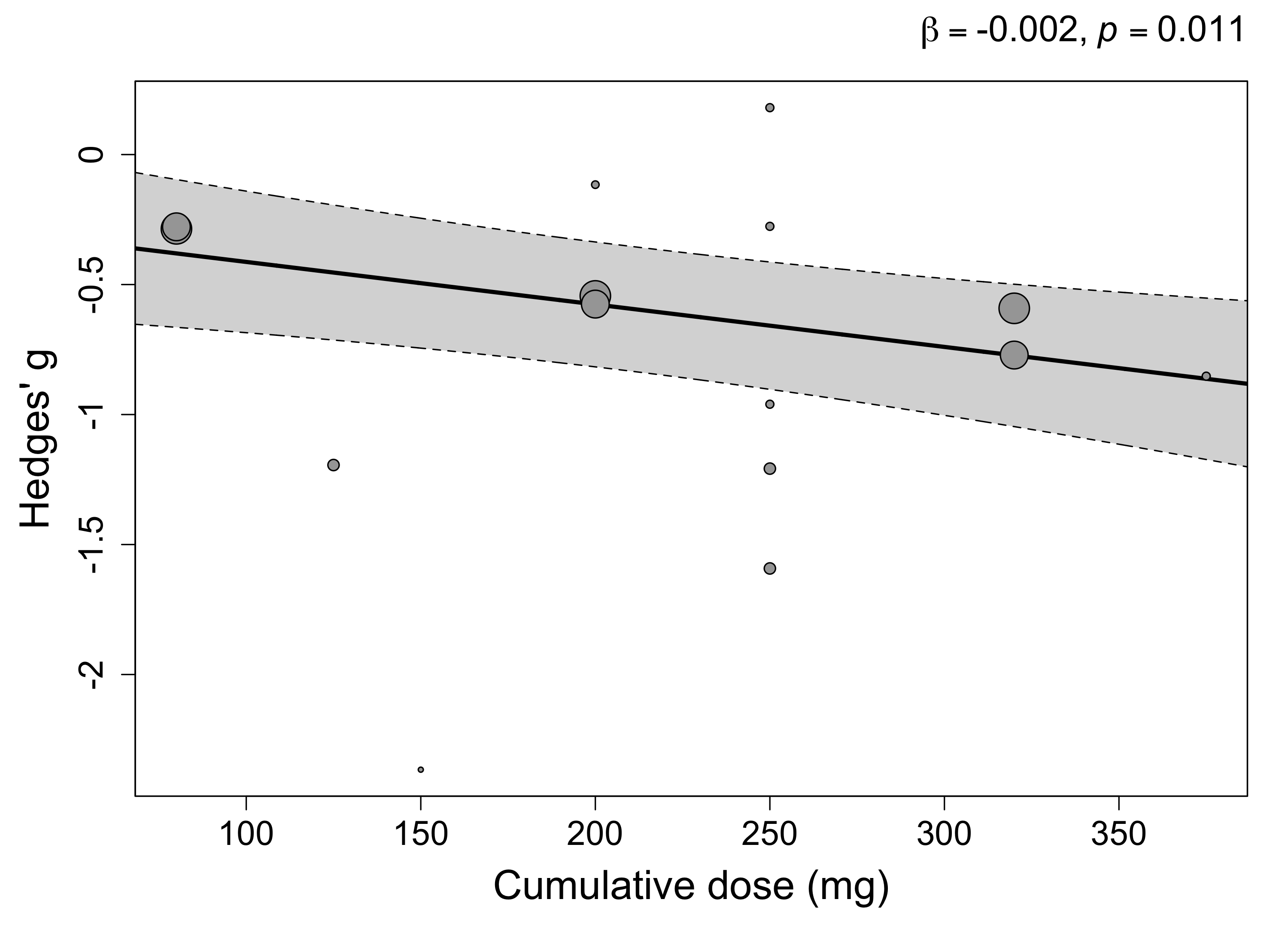
Here, while the slope is small (Hedges’ g = -0.002), this is per mg of MDMA. This comes out to about -0.20 SMD per 100 mg of MDMA.
Secondary outcomes
In addition to continuous PTSD severity scores, we also analyze dichotomous outcomes including response and remission rates of PTSD scores and secondary continuous self-reported depression outcomes. These analyses provide complementary information about the clinical significance of MDMA treatment.
Response Rate Analysis
We first analyze response rates, defined as the proportion of participants achieving a clinically meaningful reduction in PTSD symptoms.
# Get response data
data_response <- data %>%
  filterPoolingData(
    primary_instrument == "1",
    primary_timepoint == "1",
    is.na(post_crossover) | !Detect(post_crossover, "1"),
    outcome_type == "response",
    !(Detect(study, "Mithoefer 2018") & (!is.na(multi_arm1)) & Detect(multi_arm2, "75 mg")),
    !(Detect(study, "Mithoefer 2018") & (Detect(multi_arm1, "75 mg") & !is.na(multi_arm2))),
    !(Detect(study, "Ot'alora 2018") & (!is.na(multi_arm1)) & Detect(multi_arm2, "100 mg")),
    !(Detect(study, "Ot'alora 2018") & (Detect(multi_arm1, "100 mg") & !is.na(multi_arm2)))
  )

# Run meta-analysis

response_results <- runMetaAnalysis(data_response,
  which.run = "overall",
  es.measure = "RR", # risk ratio
  es.type = "raw",
  method.tau = "PM",
  method.tau.ci = "Q-Profile",
  hakn = TRUE, # Knapp-Hartung adjustement

  # Specify variables
  study.var = "study",
  arm.var.1 = "condition_arm1",
  arm.var.2 = "condition_arm2",
  measure.var = "instrument",
  w1.var = "n_arm1",
  w2.var = "n_arm2",
  time.var = "time_weeks",
  round.digits = 2
)

summary(response_results$model.overall)
##                    RR            95%-CI %W(random)
## Mitchell 2021  1.4172 [1.0766;  1.8655]       39.7
## Mitchell 2023  1.2533 [0.9967;  1.5760]       57.1
## Mithoefer 2018 2.3333 [0.6768;  8.0449]        2.0
## Oehen 2013     4.7647 [0.3237; 70.1253]        0.4
## Ot'alora 2018  3.0000 [0.4594; 19.5923]        0.9
##
## Number of studies: k = 5
## Number of observations: o = 222 (o.e = 126, o.c = 96)
## Number of events: e = 155
##
##                          RR           95%-CI    t p-value
## Random effects model 1.3494 [1.0985; 1.6577] 4.04  0.0156
## Prediction interval         [1.0559; 1.7245]
##
## Quantifying heterogeneity (with 95%-CIs):
##  tau^2 = 0 [0.0000; 1.6831]; tau = 0 [0.0000; 1.2973]
##  I^2 = 0.0% [0.0%; 79.2%]; H = 1.00 [1.00; 2.19]
##
## Test of heterogeneity:
##     Q d.f. p-value
##  2.82    4  0.5892
##
## Details of meta-analysis methods:
## - Inverse variance method
## - Paule-Mandel estimator for tau^2
## - Q-Profile method for confidence interval of tau^2 and tau
## - Calculation of I^2 based on Q
## - Hartung-Knapp adjustment for random effects model (df = 4)
## - Prediction interval based on t-distribution (df = 4)
## - Continuity correction of 0.5 in studies with zero cell frequencies
# Create simple forest plot of response results

meta::forest(
  response_results$model.overall,
  sortvar = response_results$model.overall$data$year,
  xlab = "Log RR (95% CI)",
  leftlabs = c("Study", "Log RR"),
  layout = "JAMA"
)
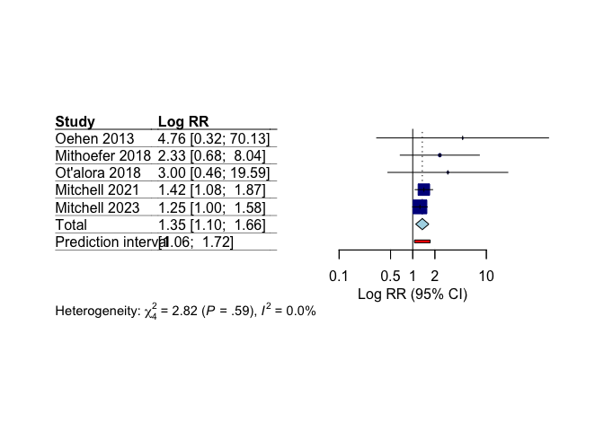
Our meta-analysis shows statistically significant greater treatment response with MDMA compared to control conditions.
Remission Rate Analysis
We also analyze remission rates, defined as the proportion of participants achieving full remission of depressive symptoms.
# Get remission data
data_remission <- data %>%
  filterPoolingData(
    primary_instrument == "1",
    primary_timepoint == "1",
    is.na(post_crossover) | !Detect(post_crossover, "1"),
    outcome_type == "remission",
    !(Detect(study, "Mithoefer 2018") & (!is.na(multi_arm1)) & Detect(multi_arm2, "75 mg")),
    !(Detect(study, "Mithoefer 2018") & (Detect(multi_arm1, "75 mg") & !is.na(multi_arm2))),
    !(Detect(study, "Ot'alora 2018") & (!is.na(multi_arm1)) & Detect(multi_arm2, "100 mg")),
    !(Detect(study, "Ot'alora 2018") & (Detect(multi_arm1, "100 mg") & !is.na(multi_arm2)))
  )

# Run meta-analysis

remission_results <- runMetaAnalysis(data_remission,
  which.run = "overall",
  es.measure = "RR", # risk ratio
  es.type = "raw",
  method.tau = "PM",
  method.tau.ci = "Q-Profile",
  hakn = TRUE, # Knapp-Hartung adjustement

  # Specify variables
  study.var = "study",
  arm.var.1 = "condition_arm1",
  arm.var.2 = "condition_arm2",
  measure.var = "instrument",
  w1.var = "n_arm1",
  w2.var = "n_arm2",
  time.var = "time_weeks",
  round.digits = 2
)

summary(remission_results$model.overall)
##                    RR            95%-CI %W(random)
## Mitchell 2021  6.1667 [1.4993; 25.3635]       12.3
## Mitchell 2023  2.1538 [1.1252;  4.1228]       58.2
## Mithoefer 2018 2.0417 [0.5762;  7.2349]       15.3
## Ot'alora 2018  1.2500 [0.3357;  4.6549]       14.2
##
## Number of studies: k = 4
## Number of observations: o = 210 (o.e = 118, o.c = 92)
## Number of events: e = 65
##
##                          RR           95%-CI    t p-value
## Random effects model 2.2499 [1.0401; 4.8667] 3.34  0.0442
## Prediction interval         [1.0066; 5.0289]
##
## Quantifying heterogeneity (with 95%-CIs):
##  tau^2 = 0 [0.0000; 5.7817]; tau = 0 [0.0000; 2.4045]
##  I^2 = 0.0% [0.0%; 84.7%]; H = 1.00 [1.00; 2.56]
##
## Test of heterogeneity:
##     Q d.f. p-value
##  2.76    3  0.4301
##
## Details of meta-analysis methods:
## - Inverse variance method
## - Paule-Mandel estimator for tau^2
## - Q-Profile method for confidence interval of tau^2 and tau
## - Calculation of I^2 based on Q
## - Hartung-Knapp adjustment for random effects model (df = 3)
## - Prediction interval based on t-distribution (df = 3)
# Create simple forest plot of remission results

meta::forest(
  remission_results$model.overall,
  sortvar = remission_results$model.overall$data$year,
  xlab = "Log RR (95% CI)",
  leftlabs = c("Study", "Log RR"),
  layout = "JAMA"
)
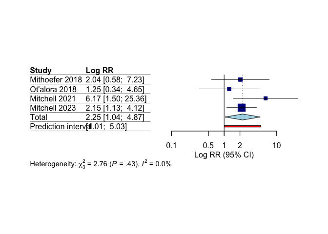
Our meta-analysis shows statistically significant higher remission rates with MDMA compared to control conditions.
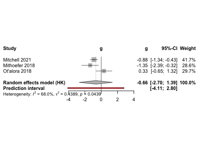
Secondary outcome - depression
Our depression outcomes are stored on a separate local database.
data2 <- read_csv("~/Documents/GIT/psypres/MDMAPTSD/data/data.csv") # for parker
## Rows: 183 Columns: 65
## ── Column specification ────────────────────────────────────────────────────────────────────────────────────
## Delimiter: ","
## chr (30): study, condition_arm1, condition_arm2, multi_arm1, multi_arm2, outcome_type, instrument, ratin...
## dbl (35): primary_instrument, time_days, time_weeks, primary_timepoint, post_crossover, n_arm1, mean_arm...
##
## ℹ Use `spec()` to retrieve the full column specification for this data.
## ℹ Specify the column types or set `show_col_types = FALSE` to quiet this message.
# data2 <- read_csv("/Users/bsevchik/Documents/GitHub/psypres/MDMAPTSD/data/data.csv") # for brooke
data2 <- data2 %>%
  calculateEffectSizes(
    vars.for.id = c(
      "study", "outcome_type",
      "instrument", "study_time_point",
      "time_weeks",
      "rating"
    ),
  )
## - [OK] Hedges' g calculated successfully.
## - [OK] Log-risk ratios calculated successfully.
# Select depression data
data_depression <- data2 %>%
  filterPoolingData(
    primary_timepoint == "1",
    is.na(post_crossover) | !Detect(post_crossover, "1"),
    !(Detect(study, "Mithoefer 2018") & (!is.na(multi_arm1)) & Detect(multi_arm2, "75 mg")),
    !(Detect(study, "Mithoefer 2018") & (Detect(multi_arm1, "75 mg") & !is.na(multi_arm2))),
    !(Detect(study, "Ot'alora 2018") & (!is.na(multi_arm1)) & Detect(multi_arm2, "100 mg")),
    !(Detect(study, "Ot'alora 2018") & (Detect(multi_arm1, "100 mg") & !is.na(multi_arm2))),
    Detect(instrument_symptom, "depression"),
    outcome_type == "msd"
  ) %>%
  filterPriorityRule(instrument = c("bdi-ii", "bid-1a", "bdi", "qids-sr", "hads-d", "smdds", "hads"))

# Run meta-analysis
dep_results <- runMetaAnalysis(data_depression,
  which.run = c("overall"),
  # Specify statistical parameters
  es.measure = "g", # Hedges' g
  method.tau = "REML",
  method.tau.ci = "Q-Profile", # N/A for three-level models
  # i2.ci.boot = TRUE, # Need to use bootstrapping to get het. CI on three-level
  hakn = TRUE, # Knapp-Hartung adjustment

  # Specify variables
  study.var = "study",
  arm.var.1 = "condition_arm1",
  arm.var.2 = "condition_arm2",
  measure.var = "instrument",
  w1.var = "n_arm1",
  w2.var = "n_arm2",
  time.var = "time_days",
  round.digits = 2
)
## - Running meta-analyses...
## - [OK] Using Hedges' g as effect size metric...
## - [OK] Calculating overall effect size... DONE
summary(dep_results$model.overall)
##                      g             95%-CI %W(random)
## Mitchell 2021  -0.8845 [-1.3415; -0.4275]       41.7
## Mithoefer 2018 -1.3503 [-2.3852; -0.3155]       28.6
## Ot'alora 2018   0.3333 [-0.6533;  1.3199]       29.7
##
## Number of studies: k = 3
##
##                                 g            95%-CI     t p-value
## Random effects model (HK) -0.6564 [-2.6982; 1.3855] -1.38  0.3008
## Prediction interval               [-4.1104; 2.7977]
##
## Quantifying heterogeneity (with 95%-CIs):
##  tau^2 = 0.4389 [0.0000; 29.5973]; tau = 0.6625 [0.0000; 5.4403]
##  I^2 = 68.0% [0.0%; 90.7%]; H = 1.77 [1.00; 3.28]
##
## Test of heterogeneity:
##     Q d.f. p-value
##  6.25    2  0.0439
##
## Details of meta-analysis methods:
## - Inverse variance method
## - Restricted maximum-likelihood estimator for tau^2
## - Q-Profile method for confidence interval of tau^2 and tau
## - Calculation of I^2 based on Q
## - Hartung-Knapp adjustment for random effects model (df = 2)
## - Prediction interval based on t-distribution (df = 2)
# Create simple forest plot of results

plot(
  dep_results,
  which = "overall"
)
## - [OK] Generating forest plot ('overall' model).
Sensitivity Analyses
We conduct comprehensive sensitivity analyses to examine the robustness of our findings.
These analyses include:
-
In the multi-arm studies (Mithoefer 2018 and Ot’alora 2018) replace high-dose intervention with medium-dose intervention
-
Fixed-effects models for primary continuous outcomes and response and remission rates
-
A Bayesian analysis of our primary results
-
Within-study correlation coefficient sweep for three-level CHE model
Medium dose comparison and fixed effects analyses
# Build a dataframe for the first sensitivity analysis
data_medium_dose <- data %>%
  filterPoolingData(
    primary_instrument == "1",
    primary_timepoint == "1",
    is.na(post_crossover) | !Detect(post_crossover, "1"),
    outcome_type == "msd",
    !(Detect(study, "Mithoefer 2018") & (!is.na(multi_arm1)) & Detect(multi_arm2, "125 mg")),
    !(Detect(study, "Mithoefer 2018") & (Detect(multi_arm1, "125 mg") & !is.na(multi_arm2))),
    !(Detect(study, "Ot'alora 2018") & (!is.na(multi_arm1)) & Detect(multi_arm2, "125 mg")),
    !(Detect(study, "Ot'alora 2018") & (Detect(multi_arm1, "125 mg") & !is.na(multi_arm2)))
  )
Now we can use metapsyTools replacement functions for quickly looking
running some sensitivity analyses.
# Use metapsyTools' replacement and rerun functions for quickly changing parameters
medium <- main_results # copy the main model
data(medium) <- data_medium_dose # replace the dataframe in the new model
medium <- rerun(medium) # re-run the model
medium
## Model results ------------------------------------------------
## Model       k     g g.ci          p        i2 i2.ci   prediction.ci   nnt
## .75 [-1.19; -0.3] 0.008  37.2 [0; 75] [-1.1; -0.39]  3.81
# Create simple forest plot of results
plot(
  medium,
  which = "overall"
)
fixed_continuous <- main_results
method.tau(fixed_continuous) <- "FE" # for this sensitivity analysis, we keep data the same but change parameters
hakn(fixed_continuous) <- FALSE
fixed_continuous <- rerun(fixed_continuous)
fixed_continuous
## Model results ------------------------------------------------
## Model       k     g g.ci           p         i2 i2.ci      prediction.ci    nnt
## .71 [-0.98; -0.45] <0.001     0 [0; 74.62] [-1.06; -0.37]  4.03
fixed_response <- response_results
method.tau(fixed_response) <- "FE"
hakn(fixed_response) <- FALSE
fixed_response <- rerun(fixed_response)
fixed_response
## Model results ------------------------------------------------
## Model       k    rr rr.ci       p         i2 i2.ci     prediction.ci   nnt
## .44 [1.2; 1.74] <0.001     0 [0; 79.2] [1.06; 1.72]   3.96
fixed_remission <- remission_results
method.tau(fixed_remission) <- "FE"
hakn(fixed_remission) <- FALSE
fixed_remission <- rerun(fixed_remission)
fixed_remission
## Model results ------------------------------------------------
## Model       k    rr rr.ci        p         i2 i2.ci      prediction.ci   nnt
## .49 [1.52; 4.09] <0.001     0 [0; 84.69] [1.01; 5.03]   3.98
Our medium dose comparison yielded similar results to the high dose comparison. Our fixed effects models yielded results that were in line with the random effects models.
Bayesian implementation
We implement our main model using a bayesian framework. We do this using
the bayesmeta package using “weakly informative prior distributions”.
Parameters: - A normal prior distribution with a 95% probability that the pooled estimate falls between -2 and 2. - A half-normal prior distribution for tau, with an s.d. of 0.5
bayes <- bayesmeta(
  data_main$.g,
  data_main$.g_se,
  mu.prior = c("mean" = 0, "sd" = 1), # asserts a 95% prior b/n -2 and 2
  tau.prior = function(t) dhalfnormal(t, scale = 0.5)
)
bayes
##  'bayesmeta' object.
##
## 6 estimates:
## 01, 02, 03, 04, 05, 06
##
## tau prior (proper):
## function (t)
## dhalfnormal(t, scale = 0.5)
## <bytecode: 0x78119fa10>
##
## mu prior (proper):
## normal(mean=0, sd=1)
##
## ML and MAP estimates:
##              tau         mu
## ML joint       0 -0.7119295
## ML marginal    0 -0.7208372
## MAP joint      0 -0.6992008
## MAP marginal   0 -0.7035442
##
## marginal posterior summary:
##                 tau         mu
## mode      0.0000000 -0.7035442
## median    0.1520771 -0.7044605
## mean      0.1921266 -0.7047483
## sd        0.1614149  0.1759992
## 95% lower 0.0000000 -1.0545489
## 95% upper 0.5087099 -0.3574634
##
## (quoted intervals are shortest credible intervals.)
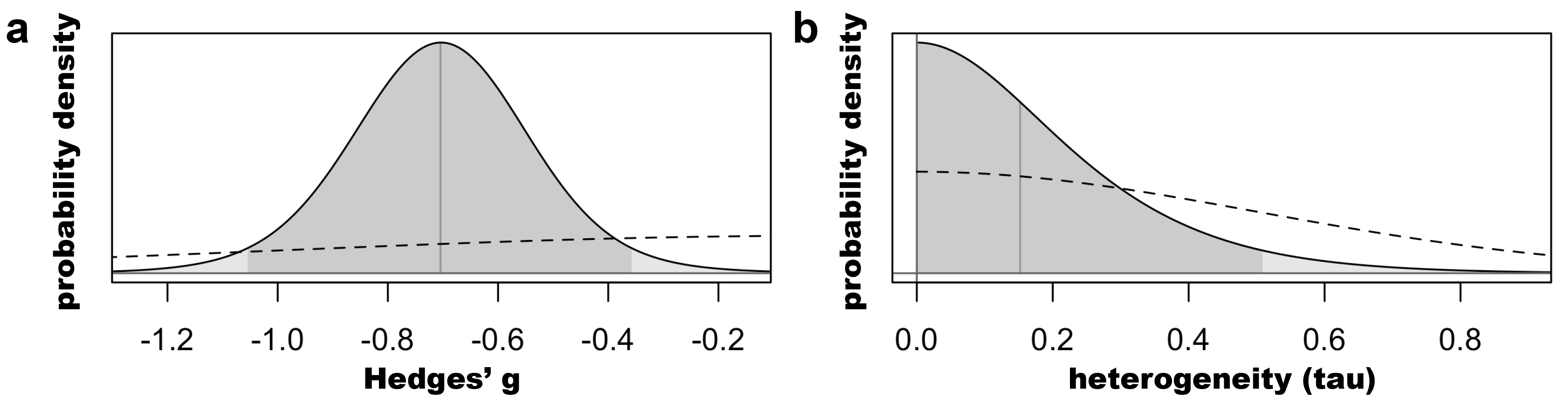
Above we can see the characteristics of the marginal posterior distributions of tau and mu (the pooled estimate). The model finds that the 95% interval of the true effect lies between -1.05 and -0.36.
We can visualize each posterior probability distribution (solid line),
along with the priors (dashed) below:
Sweep the within-study correlation coefficient for the three-level CHE
The CHE model assumes that there is a known correlation “rho” between effect sizes in the same study; and that “rho” has the same value within and across all studies in our meta-analysis (the “constant sampling correlation” assumption, J. E. Pustejovsky and Tipton 2021). While these authors have reported that “meta-regression coefficient estimates were largely insensitive to assuming different values of rho between 0.0 and 0.8”, our default choice of rho = 0.6 in metapsyTools is nonetheless, a guess. It is therefore generally recommended to run sensitivity analyses for varying values of rho:
# sweep rho in the CHE model for r = seq(0, 1, 0.1)
rho_seq <- seq(0, 1, 0.1)
i <- 1
g_sweep <- numeric(length(rho_seq))
g_ci_lwr <- numeric(length(rho_seq)) # Initialize the vector
g_ci_upr <- numeric(length(rho_seq)) # Initialize the vector

for (rho in rho_seq) {
  time_results_sweep <- runMetaAnalysis(data_time,
    which.run = "threelevel.che",
    # Specify statistical parameters
    es.measure = "g", # Hedges' g
    method.tau = "REML",
    method.tau.ci = "Q-Profile", # N/A for three-level models
    hakn = TRUE, # Knapp-Hartung adjustment
    rho.within.study = rho,
    # Specify variables
    study.var = "study",
    arm.var.1 = "condition_arm1",
    arm.var.2 = "condition_arm2",
    measure.var = "instrument",
    w1.var = "n_arm1",
    w2.var = "n_arm2",
    time.var = "time_days",
    round.digits = 2
  )

  g_sweep[i] <- time_results_sweep$summary$g[2]
  g_ci <- as.numeric(
    strsplit(gsub("\\[|\\]", "", time_results_sweep$summary$g.ci[2]), ";")[[1]]
  )
  g_ci_lwr[i] <- g_ci[1]
  g_ci_upr[i] <- g_ci[2]
  i <- i + 1
}
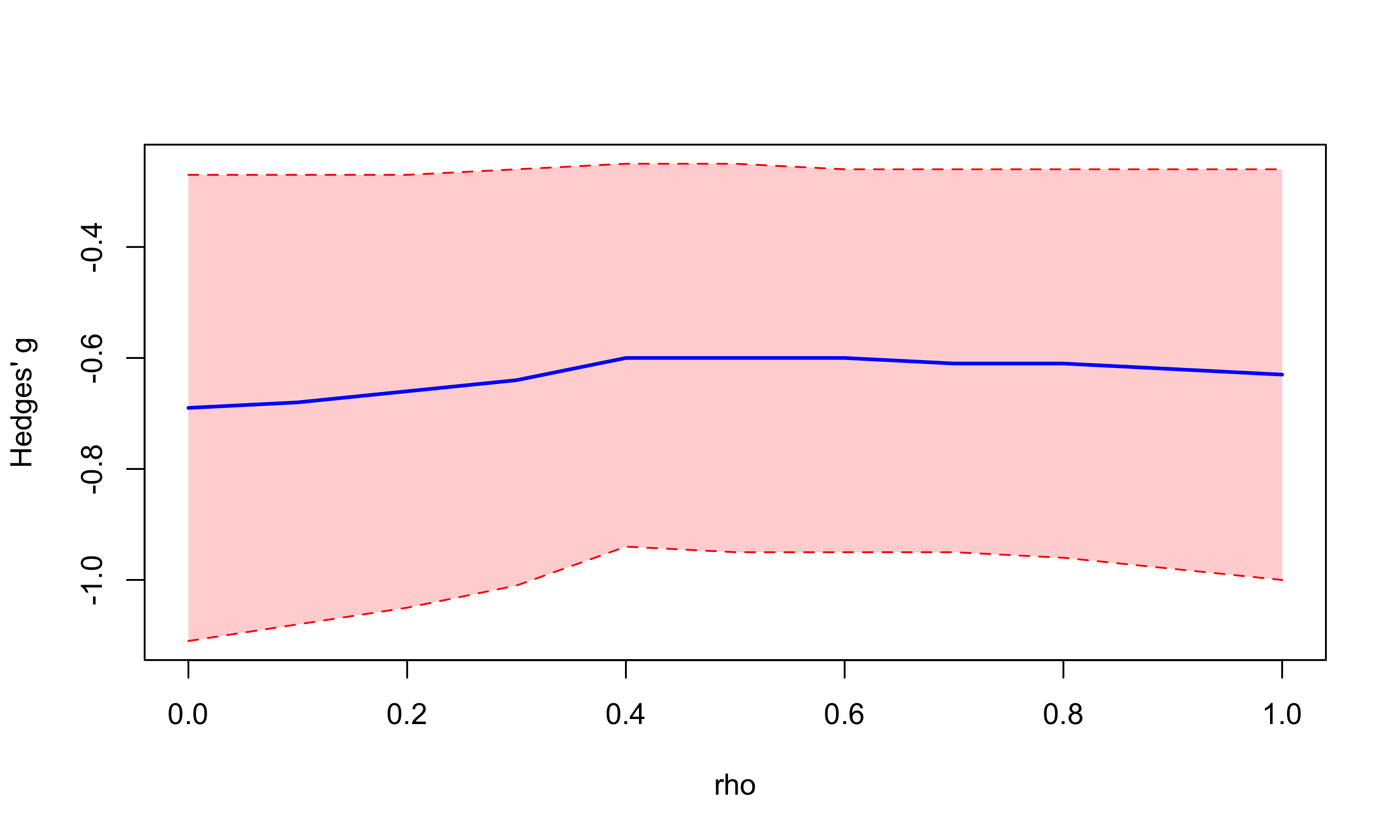
The main effect size is not sensitive to the within-study correlation coefficient.
Summary and Conclusions
This comprehensive meta-analysis provides promising evidence regarding the efficacy of MDMA for treating PTSD, but should be interpreted with caution.
The analysis includes:
- Primary analysis of continuous PTSD severity outcomes using standardized mean differences
- Dose-response analysis examining how treatment effects are impacted by number of dosing sessions and cumulative dose
- Dichotomous outcomes analysis of response and remission rates
- Secondary outcomes analysis of self-reported depression outcomes
- Extensive sensitivity analyses to examine robustness
The results demonstrate consistent evidence for the efficacy of MDMA in reducing PTSD severity, with effects showing robustness across various sensitivity analyses. However, given the small number of studies eligible to include in our meta-analysis and limitations such as the potential for functional unblinding and expectancy effects, results should be interpreted with caution.